A Generalized Elo System for Tennis Players, part 2

In this notebook, we will take our previous Elo system for tennis players and add playing surface as a parameter.

This is part 2 of a 3-part series. Here is part 1 and part 3. All of the code I wrote for this project is here.

There are a few ways in which surface has been taken into account.

(Surface-only) Treat each surface as a different sport altogether, so that each player has three ratings that don’t interact with one another.
(Weighted average) Take the surface-specific ratings in item 1 above and the all-surfaces ratings developed in our previous post, then take a weighted average of them, minimizing the log-loss error.
(Surface-dependent K-factor) According to the surface being played on, update each player’s surface-specific rating according to a different K-factor and take the win probability from the corresponding surface-specific ratings.

The first and second are implemented by Jeff Sackmann, the tennis data god, where the weighted average is the actual average. (Actually on his website, he averages the raw Elo ratings themselves, but that’s fairly similar—though not identical—to what I described.) The third is the idea introduced in this post, which seems fairly natural to me and perhaps a little less ad-hoc than taking the average between surface-only and surface-agnostic ratings. So let’s explain how the surface-dependent K-factor (SDKF) model works.

Code

The code for this project is available on my GitHub.

SDKF model

Define ++\sigma(x) = \exp(x) / (\exp(x) + 1),++ the logistic function. If player one (p1) has rating $x$ and player two (p2) has rating $y$, the probability that p1 wins is given by $\sigma(x-y)$. Suppose $w=1$ if p1 wins and $w=0$ if p1 loses. After the match, the ratings are updated with the rule ++x \mapsto x + (-1)^{w+1} K(n_1)\sigma((-1)^w(x-y)),\quad y \mapsto y+(-1)^w K(n_2)\sigma((-1)^w (x-y)),++ where $K$ is a function of the number of matches played by p1 ($n_1$) and the number of matches played by p2 ($n_2$). The function $K$ is of the form ++K(n) = \frac{a}{(b + n)^c}.++

To define surface-specific ratings, we can do the following. Let $A$ be a $3\times 3$ matrix. We map surfaces to indices: index 1 refers to clay, 2 to grass, 3 to hard. Now let $\vec{x},\vec{y}\in \mathbb{R}^3$ be the ratings of p1 and p2, respectively. Specifically, ++\vec{x} = (x_1,x_2,x_3)++ and $x_1$ is the p1 clay rating, $x_2$ is the p1 grass rating, and so on. Define $\sigma(\vec{x}) = (\sigma(x_1),\sigma(x_2),\sigma(x_3))$. If $a_{ij}$ is the $(i,j)$ entry of $A$, then we make the following change to the update rule: ++\vec{x} \mapsto \vec{x} + (-1)^{w+1}K(n_1)A\sigma((-1)^w(\vec{x}-\vec{y})), \quad \vec{y} \mapsto \vec{y} + (-1)^w K(n_2)A\sigma((-1)^w(\vec{x}-\vec{y})).++

The matrix $A$ consists of the speed with which to update each of the three ratings, given the surface being played on. For example, if the match is being played on grass, we intuit that the result shouldn’t have a large effect on the players’ clay rating, but it should have a large effect on the players’ grass rating. On the other hand, if the match is being played on hard, we might think that it should have an equal effect on the players’ grass and clay ratings.

Finally, let’s determine the win probability and the interpretation of the matrix $A$. If ++\vec{s}=\begin{cases} \vec{e}_1 &\quad \text{ if clay} \\ \vec{e}_2 &\quad \text{ if grass} \\ \vec{e}_3 &\quad \text{ if hard} \end{cases}++ is the vector denoting surface being played on, then the win probability of p1 is ++\sigma(\vec{x}-\vec{y})\cdot \vec{s}.++ This indicates that $a_{ij}$ is the update speed for the players’ surface $i$ rating if the playing surface is $j$.

Special cases

It is instructive to examine special cases of $A$.

If $A$ is the identity matrix, then no surface affects any other surface, and all the update coefficients are equal. So this would be equivalent to treating each surface as a different sport altogether (Surface-only ratings).
If $A$ is the all-ones matrix, then all surfaces are treated equally. This results in surface-agnostic ratings, which is the classical setting.

Based on these two extremes, we expect an effective $A$ to have heavy diagonal entries but nonzero off-diagonal entries, all positive. For our $K$, we take $a,b,c$ to be ++(a,b,c) = (0.47891635, 4.0213623 , 0.25232273)++ based on training data from 1980 to 2014, from the previous post. Then we initialize the entries of $A$ to be uniform random numbers between 0 and 1.5.

Parameter Search

We draw 10000 samples from a uniform distribution on $A\sim [0,1.5]^9$. We get these results.

            ll        wp        bs
0.575501  0.678254  0.197409
0.575569  0.679325  0.197355
0.575620  0.679489  0.197426
0.575660  0.679572  0.197463
  0.575678  0.679489  0.197462

            a1        a2        a3        a4        a5        a6        a7  \
1.497282  0.709504  0.223734  0.035879  1.016345  0.891814  0.635505   
1.496927  0.122563  0.659796  0.035299  0.704547  1.405535  0.895188   
1.403872  0.472810  0.730792  0.233342  0.614701  1.108361  0.540628   
1.459754  0.449260  0.745738  0.556220  1.398105  0.590583  0.627694   
  1.459020  0.305191  0.589823  0.331715  1.321166  0.879316  0.332806   

            a8        a9  
1.089314  1.143836  
0.967678  1.212636  
1.486120  1.129831  
0.869944  1.246126  
  0.439226  1.318882  

We see good log-loss and heavy diagonal entries on a1, a5 and a9. We also see that a3, which is the update speed of a player’s clay rating if the playing surface is hard court, is larger than the update speed of a clay rating if the playing surface is grass. This makes total sense. So our model naturally gravitates to the common-sense heuristics. Since our parameter space is bigger now and our parameters seem to have reasonable variance, we will constrain our search to the uniform distribution centered at the mean of our top 50 parameters plus or minus 4 standard deviations. We get these results.

            ll        wp        bs
0.574072  0.679654  0.196739
0.574075  0.680478  0.196746
0.574086  0.680313  0.196760
 0.574098  0.680560  0.196769
 0.574109  0.681054  0.196764

            a1        a2        a3        a4        a5        a6        a7  \
1.383559  0.186148  0.582325  0.163048  1.366782  0.642451  0.640518   
1.367565 -0.038163  0.501433  0.141208  1.225584  0.738717  0.557209   
1.367434  0.034490  0.492734  0.135281  0.840048  0.683265  0.598902   
1.347424  0.120422  0.612078  0.116368  1.020613  0.703088  0.524921   
 1.373804  0.209944  0.514236  0.163280  1.325427  0.585647  0.450906   

            a8        a9  
1.258164  1.285806  
0.815735  1.200875  
1.250441  1.270224  
1.242716  1.166514  
 0.925887  1.271030 

A small improvement. We do have one negative value which is a little counterintuitive, but it’s small. With these parameters, which were trained on 1995-2013 data, we get the following log-loss, win prediction, and brier score (respectively) for 2014 data and for 2015-2019 data respectively.

# 2014
(0.579, 0.673, 0.199) # ours
(0.585, 0.669, 0.201) # FiveThirtyEight's

#2015-2019
(0.603, 0.664, 0.208) # ours
(0.612, 0.662, 0.211) # FiveThirtyEight's

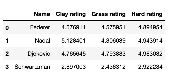
Pretty good. We are able to reduce log-loss by 1% or so from FiveThirtyEight’s model. Some sample averaged ratings are below.

Comparison with SA+SO average: a little bit of a bummer

Now let’s build a model in which the win probability is averaged between the predictions given by the surface-agnostic rating and the surface-only rating. With our framework, the respective $A$s are ++ \begin{pmatrix} 1&1&1\\1&1&1\\1&1&1\end{pmatrix}, \quad \begin{pmatrix}1&0&0\\0&1&0\\0&0&1\end{pmatrix}.++ The average method fits right into our framework and can be computed with one line of code. On 2015-2019 data, we get the following results.

(0.603, 0.661, 0.208)

The 0.603 is actually a little smaller than ours, by 0.0005. So it’s a little bit of a bummer that this rather ad-hoc method does as well as our more principled method. But that’s just life.

Conclusion

The SA+SO model still uses my hyperparameter principles from the previous notebook, and it fits quite nicely into the mathematical framework I’ve made here. If I could search for parameters like a thousand times faster, I might try to optimize for a weighted average of probabilities from two matrices, to get results like the above. With our current parameter search, we can’t find this local min because neither matrix by itself does well, but averaged together they do well. Doing this larger parameter search, we’d need to search through, in all probably, millions of parameters, which doesn’t seem all that bad, in the context of all the deep learning stuff I’m doing recently. We might even be able to do a little bit of gradient descent (which I tried earlier but it didn’t work because the loss function was so rough in the parameter space and uniformly chosen parameters all did fairly well – in this case, uniformly chosen parameters do very badly so gradient descent might work initially). So next up, I’m going to load this up in Google Colab and see if I can run it.