A Generalized Elo System for Tennis Players, part 1
Here, we will create an Elo rating system for male tennis players and do some analysis on the choice of parameters. We find that a random choice of parameters actually does quite well, and that a wide variety of K-factor weight functions do a good job predicting the outcomes of tennis matches. In future notebooks, we will further expand upon this model by adding various features.
This is part 1 of a 3-part series. Here is part 2 and part 3. All of the code I wrote for this project is here.
Background
The Elo rating system is designed to assign ratings to players which reflect their true strength at the game. Players are assigned an initial rating of 1. Before a match between two players, the system outputs a probability that one wins. After the match, the system updates each player’s rating according to their previous ratings and the result of the match.
Elo’s rules
Define ++\sigma(x) = \exp(x) / (\exp(x) + 1),++ the logistic function, and let $K$ be a constant. If player one (p1) has rating $x$ and player two (p2) has rating $y$, the probability that p1 wins is given by $\sigma(x-y)$. Suppose $w=1$ if p1 wins and $w=0$ if p1 loses. After the match, the ratings are updated with the rule ++x \mapsto x + (-1)^{w+1} K\sigma((-1)^w(x-y)),\quad y \mapsto y+(-1)^w K\sigma((-1)^w (x-y)).++
Deriving Elo’s rules
Let’s see why this makes any sense. Suppose we are starting from scratch and we want to develop this kind of rating system, but have no idea what the win probability and the update rule should be. Heuristically, it makes sense to suppose that $W,U$ are functions of the difference $x-y$ rather than the separate ratings $x,y$. Let $W(x-y)$ be the probability that p1 wins against p2, and let $U(x-y)$ be the update rule if p1 loses and $U(y-x)$ be the update rule if p1 wins, so that ++ x\mapsto x+(-1)^{w+1} U((-1)^w(x-y)),\quad y\mapsto y+(-1)^w U((-1)^w(x-y)).++ We need $W$ and $U$ to satisfy some basic rules.
First, $W(x-y) = 1-W(y-x)$ so ++W(z)+W(-z)=1.++
Second, ++\lim_{x\to \infty} W(x)=1 ~\text{ and }~ \lim_{x\to-\infty} U(x) = 0.++
Third and last, the expected update of both players must be zero. This is because the strengths of the players shouldn’t actually change after a match, so the Elo rating (which is supposed to reflect true strength) shouldn’t do that. Here, $w$ is the random quantity in question (make sure to distinguish between little $w$ and capital $W$: the relationship is that $W(x-y)$ should estimate $P(w=1)$). Since the expected update of both players equals zero, we have ++ W(x-y) \cdot U(y-x) - W(y-x) \cdot U(x-y) = 0. ++ In other words, ++ \frac{W(z)}{W(-z)} = \frac{U(z)}{U(-z)}.++ In fact, these are the only real mathematical requirements for such a rating system. (See Aldous for more details and assumptions.) As we see, an easy choice would be to set $KW=U$, where $K$ is any constant greater than zero. And really we may set $W$ to be any cdf, but logistic is the standard choice.
In practice, the choice of $K$ is quite important, and the constant is called the K-factor, not to be confused with the tennis racquet line. This $K$ is the main subject of this note, and we will refer to it many times.
Generally $K$ is taken to be a decreasing function of the number of matches that the updating player has played. In our case, following FiveThirtyEight’s family of functions for $K$, we take ++K(n) = \frac{a}{(b+n)^c},++ where $n$ is the number of matches played by that player before the match. We will call $K(n)$ the K-factor function. All of the analysis of parameters we do below focus on the parameters $a,b,c$ above.
We will use Jeff Sackmann’s immense trove of tennis data; see his GitHub page.
Differences with standard Elo ratings
You may notice that I chose to work with the natural base rather than base-10 with some weird 400 multiplicative factor like with standard Elo ratings. The only difference between my ratings and the ratings you may see on FiveThirtyEight or Jeff Sackmann’s website is a multiplicative factor of $400/\ln 10\approx 173.72$. There is also an additive factor, but we can ignore that because Elo ratings give the same predictions when the same value is added to all ratings (and all initial ratings). We explain the origin of the multiplicative factor below.
For the standard Elo rating, the win probability of player with rating $x$ (who is facing a player with rating $y$) is ++ \frac{1}{1+10^{(y-x)/400}} = \frac{1}{1+ \exp\left(\frac{\ln 10}{400}(y-x)\right)} ++ So we have to multiply our ratings by $400/\ln 10\approx 173.72$ to get the standard Elo ratings. There’s also an additive factor of $1000-173.72$ because generally the tennis ratings start at 1000, and we start at 1.
Cost functions
There are many ways to measure the accuracy of a prediction model which outputs probabilities. Let $n$ be the number of matches being analyzed and $p_i$ the win probability that the model assigns to the winner for $i=1,2,\ldots,n$.
The easiest to understand is win prediction rate, which is simply the proportion of matches for which the model assigns a probability greater than 0.5 to the winner. In the code, win prediction rate is denoted by wp. Below, $\mathbb{1}(A)=1$ if $A$ happens and $\mathbb{1}(A)=0$ if $A$ does not happen. Technically this is not a cost function, it’s a profit function. Take the negative of this if you want a cost function.
++\text{wp} = n^{-1}\sum_{i=1}^n \mathbb{1}\{p_i > 0.5\}.++
Next, we introduce log-loss error, appearing in maximum likelihood estimation and logistic regression. In the code, log-loss error is denoted by ll.
++\text{ll} = -n^{-1}\sum_{i=1}^n \log p_i.++
Finally, we introduce the Brier score, which is simply the mean squared error between $p_i, i=1,2,\ldots,n$ and the perfect data which assigns probability one to the winner every time. In the code, Brier score is denoted by bs.
++\text{bs} = n^{-1} \sum_{i=1}^n (1-p_i)^2.++
Here are some apparent differences between these cost/profit functions.
- win prediction rate is not continuous (a small change in probabilities can change 0s to 1s and 1s to 0s) and also flat in many places (with respect to the parameters), so it is less useful for optimization than the other two functions, though still a nice metric.
- log-loss is not bounded, while Brier score is. To see the difference, suppose $p_1=10^{-100}$. Then this contributes 230 to the log-loss error, while it contributes 1 to the Brier score. So log-loss is less tolerant of wrongly confident predictions.
Let’s first look at FiveThirtyEight’s model, described in a very nice article about Serena Williams’ dominance over the years.
FiveThirtyEight’s model
FiveThirtyEight’s parameter choices were ++[a,b,c]=[250/174, 5, 0.4] \approx [1.44, 5, 0.4].++ Let’s test their model on 2014 data with one year of history and 34 years of history.
One year of history:
log-loss=0.601, win pred=0.650, brier score=0.209
many years of history:
log-loss=0.585, win pred=0.669, brier score=0.201
I got the same log-loss error that Kovalchik got, but I got a different win prediction. I’m not entirely certain how that happened, since I think we used the same data set. I’m gonna have to go on with what I have.
Sensitivity of Ratings
Recall that the parameters we are interested in are the ones which dictate the behavior of the K-factor function. My main observation for this post is that ratings are not very sensitive to the parameters because 1) the model itself is pretty robust, and 2) there are some redundancies in our three parameters. By this, I mean that very different sets of parameters can produce similar K-factor functions.
We will initialize an object of class Elo with parameters $p$ which are obtained from the following distribution:
++ p \sim \text{Unif}([0,2]\times[2,5]\times[0,1]). ++
We will calculate and plot log-loss error, win prediction rate, and Brier score for 100 models with random parameters drawn from the above distribution. To do this fast, we need to modify our class to accommodate vectorized operations. We change our code so that ratings according to different parameters are all updated simultaneously.
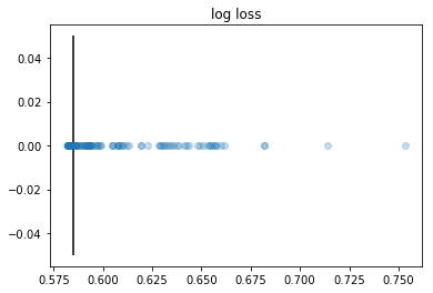
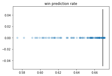
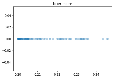
The conclusion is that most parameters drawn from this simple uniform distribution do pretty well. The parameter population is the densest where the best costs are achieved. In other words, good parameters are not rare. Recall that log-loss=0.585, win pred=0.669, brier score=0.201 were the costs achieved by the handpicked FiveThirtyEight parameters. The plots have vertical lines at these checkpoints.
You bring your best fifty, I’ll bring mine
How good are the best parameters from these randomly chosen ones? Let’s pick the top 1% of parameters and see how they perform. I will pick the 50 best parameters (tested on 2010-2013) in each of the three categories from 5000 random ones with 1990-2013 data. Then we test them on 2014 data. For each category, to get a single probability, we took the 50 probabilities generated by the 50 models and averaged them.
  optimized_for        ll        wp        bs
0            ll  0.581776  0.670516  0.199910
1            wp  0.595646  0.666440  0.204376
2            bs  0.581727  0.669497  0.199868
We see that the parameters which were obtained by optimizing for log-loss and Brier score were about equally effective at predicting 2014 matches, and the win-prediction-optimized parameters were less effective. But overall, all of these parameters are not bad. What do these parameters look like? Are they clustered anywhere? Are they all over the place? Recall the roles of the first, second, and third parameters, below denoted by $a,b,c$: ++k(n) = \frac{a}{(b+n)^c}.++
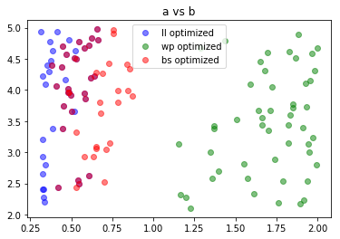
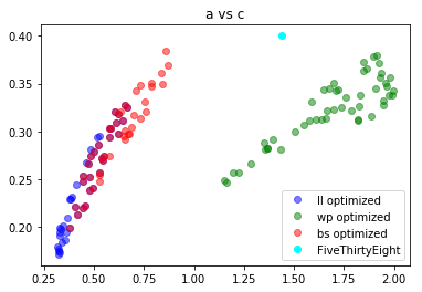
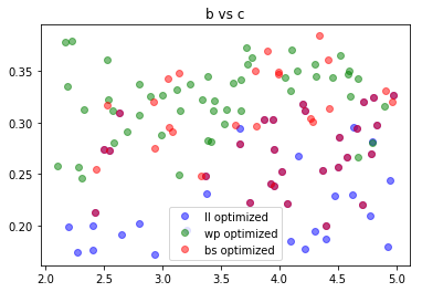
From these plots, we can see that basically b doesn’t matter, and based on the type of error optimized for, the parameters cluster around different pairs of $(a,c)$ values. There is some overlap between the log-loss optimized parameters and the Brier-score optimized parameters, as evidenced by the purple points.
The correlation in the second plot is due to the fact that, for a fixed $n,a,b,$ and $c$, the set of points $(x,y)$ satisfying ++\frac{x}{(b+n)^y} = \frac{a}{(b+n)^c}++ is a log curve.
In short, there are a variety of parameter choices that can lead to effective predictions. All of the parameters shown above achieve pretty good error rates.
You may be wondering if maybe, two sets of parameters could be quite different as points in 3-d space but give rise to two very similar k-factor functions $k(n)$. This is true, as evidenced by the clustering around a log curve shown above. Our tentative conclusion is that parameters within a single group (that is, optimized for the same cost function) give rise to similar K-factor functions, but the three different groups (ll-optimized,wp-optimized,bs-optimized) give rise to fairly different K-factor functions.
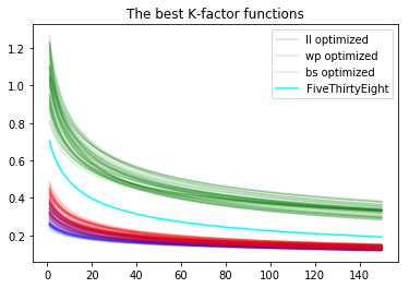
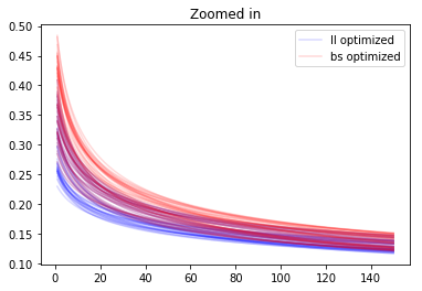
It seems clear that the differently colored K-factor functions behave quite differently, both near zero and at infinity.
Testing on 2015-2019 data
The ll-optimized and bs-optimized parameters (trained on 1980-2013) performed a tiny better than the FiveThirtyEight model with respect to each of the three cost functions for 2014 data. What about for 2015-2019 data? We’ll check it out here.
  optimized_for        ll        wp        bs
0            ll  0.607112  0.658860  0.209942
1            wp  0.623405  0.657555  0.214121
2            bs  0.607411  0.658723  0.209912
3           538  0.611903  0.661607  0.210791
FiveThirtyEight takes the highest win prediction rate. On the other hand, the ll- and bs-optimized parameters achieve the best log-loss errors. Overall, aside from wp-optimized parameters, all of these models seem to give roughly equally effective predictions. (This discrepancy is explained by the fact that mathematically, wp is not nice to work with because it is flat and discontinuous.)
Conclusion
First, this analysis casts doubt on my initial feeling that there is one “true” K-factor function that we wish to approximate. It seems that many quite different K-factor functions can be used for effective and near-optimal prediction, given this model.
Second, I believe that a random choice of parameters is a better one than a handpicked one, from an algorithmic point of view. It separates the parameters from most human fiddling (except the distribution that we pick from, which was pretty generic – a uniform distribution on a large 3-d box).
Third, the fact that many different K-factor functions work opens up a new frontier of prediction with Elo. Can we use, say, ten different Elo models at once to make a better prediction than any one of them can? Perhaps we can use a fast-updating Elo model in conjunction with a slow-updating Elo model to generate more effective predictions. We will explore these ideas and more in the next notebook.