A Visual Introduction to Interacting Particle Systems
An interacting particle system is a stochastic process in which particles randomly move around as time passes with certain exclusion rules. Here, we explain some problems and ideas in interacting particle systems literature.
One Particle System
Suppose you have one particle on the integer number line. You flip a coin, and if it’s heads, the particle jumps left; if it’s tails, the particle stays. Keep flipping coins. This simple one-particle-model looks like this when simulated. The $t$ denotes the $t$th coin flip, and the variable $t$ stands for time.

The main question we ask is: what is the long-term behavior of the particle? By “long-term,” I mean: if a long time passes, what can we say about where the particle is?
Suppose the starting point of the particle is zero. At time $t$, the position of the particle is ++ p(t) = -(X_1 + X_2 +\cdots + X_t), ++ where ++ X_i =\begin{cases}
1 &\quad \text{if heads} \
0 &\quad \text{if tails}
\end{cases} ++
represents the result of the $i$th coin flip. This formula gives us all that we can possibly know about the long-term behavior of $p(t)$ because sums of independent coin flips are possibly the most-studied object in probability.
- We know, for example, that ++ \lim_{t\to \infty} \frac{p(t)}{t} = \frac{-1}{2}, ++ where the limit is interpreted in basically any fashion.
- We also know that ++ \frac{p(t) + t/2}{\sqrt{t}/2} \text{ is approximately } N(0,1), ++ the standard normal distribution.
The first of these is called the Law of Large Numbers (LLN), and the second is called the Central Limit Theorem (CLT). They are cornerstones of probability theory.
Many-particle system with interaction
With one particle on the number line, classical probability theory can easily answer any question about the long-term behavior of the system. What if there are many particles on the number line?
If there are many particles and the particles can pass through one another without consequence, then each particle behaves independently of the others. We effectively get many copies of the one-particle system explored in the previous section.
In our physical world, particles interact with one another. They bounce off of each other like billiards balls, or they might attract or repel one another. The simplest model for particle repulsion is to disallow particles occupying the same space.
Let’s expand our single-particle system to accommodate many particles. Each particle has a coin above it which gets flipped at every time step. All the coins flip simultaneously. If the coin lands heads, the corresponding particle tries to jump one spot to the left. However, if the left-neighboring spot is occupied, the particle does not jump. If the coin lands head and the left-neighoring spot is unoccupied, the particles jumps left.

This simple particle interaction rule adds a ton of complexity to the model. This model is called the totally asymmetric simple exlusion process (TASEP). “Totally asymmetric” because particles only jump to the left, “exclusion” because we exclude particles occupying the same position, and “simple” because… it’s the simplest of these kind of interacting particle systems?
The resolution of the analogue of the CLT for particle systems like these is an enormous challenge in probability. LLN is generally easier and verified for larger classes of particle systems, but the CLT is very difficult, and only resolved in specific models like TASEP. And even for TASEP, there is a lot to discover about its fluctuations in the CLT realm.
Height function
One of the simplest initial configurations to start with is the “wedge” initial condition, displayed in the animation above. In the setting where particles are only jumping to the left, this means that every site to the right of and including zero is occupied, while every site to the left of zero is unoccupied. Another simple initial condition is the one in which each site is occupied with probability $p$, and all sites are independent of one another. To obtain a full understanding of TASEP, we need to consider both initial conditions. And in fact, all other possible initial conditions can sort of be boiled down to these I think. For us, we will only look at the wedge initial condition.
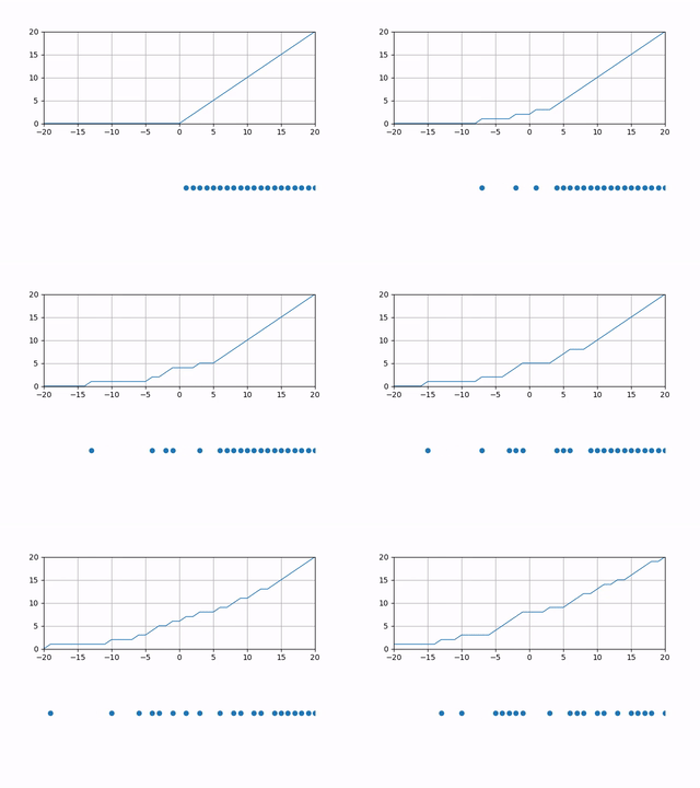
To study the dynamics, we introduce a height function corresponding to the system, which helps us analyze it. We begin with the wedge initial condition. The {\emph height function} $h(x,t)$ associated with the particle system is a function which counts the number of particles strictly to the right of $x$ at time $t$. This means that the height function starts at $h(x,0) = \max(0,x)$, which represents the wedge initial condition, and each time a particle jumps from $x$ to $x-1$, then $h(x,t)$ increments by one. Here is what $h(x,t)$ would look like as time passes.

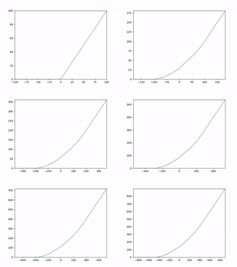
Remember that we want to study the long-term dynamics of $h(x,t)$. Just as we do for LLN when we study $X_1+X_2+\cdots+X_n$ the sum of $n$ iid random variables, we must scale by an appropriate factor while letting $t\to\infty$. The correct scaling is ++ \lim_{\epsilon \to 0} \epsilon h\left(\frac{x}{\epsilon}, \frac{t}{\epsilon}\right). ++ Essentially, when $\epsilon \to 0$, we are zooming out and speeding up time at such a rate so that we get an interesting function at the end of the limit. Here is what that would look like.

You can observe that while the microscopic dynamics are random, the macroscopic dynamics seem to be converging to a deterministic function! This is LLN for this particle system. We see it in this animation, but proving it is another matter.
You might ask, what is CLT for this particle system? It is very complicated and I myself have only barely touched the tip of the iceberg here. The analogue of the Gaussian distribution is various distributions related to the KPZ equation. TASEP is one of the simplest models in the “KPZ universality class,” which is loosely defined as a class of models for which the fluctuations are expected to follow the same distributions that the KPZ equation exhibits.
Conclusion
We will hopefully get to the kinds of things I investigated in my graduate studies. I looked at a generalization of TASEP whose fluctuations are unknown (but expected to be in the KPZ class) and derived some bounds for the fluctuations. More to come.